Diversidad socioeconómica regional de los flujos de migración interna en Brasil

 

Regional socioeconomic diversity of internal migration flows in Brazil

 

André Braz-Golgher

Denise Helena França-Marques^*

 

Abstract

 

Poverty levels in Brazil present a remarkable spatial heterogeneity. Among other phenomena, migration may also have an impact on regional poverty levels. Based on this background, we analyzed the regional socioeconomic diversity of urban/urban, rural/urban, urban/rural and rural/rural flows of migrants within and between states in Brazil. In order to do so, we applied the multivariate technique of Cluster Analysis. We observed some general tendencies, as the higher socioeconomic levels of urban/urban and distant flows, and lower socioeconomic levels for rural/rural and short step migrations. Moreover, most poor migrants were in flows with rural origin and/or destiny in the Northeast Region.

 

Keywords: migration, poverty, Brazil, Latin America.

 

 Resumen

 

Los niveles de pobreza en Brasil presentan una notable heterogeneidad espacial. Entre otros fenómenos, la migración puede tener cierto impacto en los niveles de pobreza regionales. Con estos antecedentes, se analiza la diversidad socioeconómica regional de los flujos migratorios en los siguientes casos: urbano-urbano, rural-urbano, urbano-rural y rural-rural dentro y entre los estados de Brasil. Para ello se utilizaron técnicas multivariables de análisis de clusters. Se observan algunas tendencias generales: entre mayor es el nivel socioeconomico hay mayores flujos urbano-urbano y de mayor distancia, mientras que entre menor es dicho nivel se dan más flujos rural-rural y de menor distancia. Más aún, los emigrantes más pobres se encuentran en los flujos con origen rural en y/o con destino  a la región Noreste del país.

 

Palabras clave: migración, pobreza, Brasil, Latinoamerica.

 

 

* Universidad Federal de Minas Gerais, Brasil: Correos-e: agolgher@cedeplar. ufmg.br; denise@cedeplar.ufmg.br.

 

 

Introduction

 

Poverty levels in Brazil showed a tendency of stability between 1977 and 1999 at high figures (Barros et al., 2000), and just very recently that it was verified a slight advance on these levels (ibre-fgv, 2005). Moreover, Hoffmann (2000) and Ferreira et a.l (2000) showed that poverty levels in Brazil presented a remarkable spatial heterogeneity. Among the five macroregions of this country, the Northeast Region had the greatest proportions of poor people, especially in rural areas. The North Region followed the Northeast of Brazil and also had large proportions of poor individuals. In the other macroregions of Brazil, Southeast, South and Center-West, the numbers were smaller, but still quite expressive.

There are many phenomena that may have an impact on regional poverty levels and migration is one of them. The influence of migration on poverty depends on the magnitude of the flows and also on their composition, because they may change population growth regimes, the age distribution of the population and also the regional amount of human and other types of capital.

The human capital model is a commonly used framework in economic theory to discuss issues related to migration and its´ impacts on regional features, including poverty levels. This model assumes that a rational individual migrates if the expected net return of migration is positive and if so, he/she maximizes his/her utility among the possible destinies (Stillwell and Congdon 1991). The equation below presents this relation:

 

(1)  G_ij = (V_ij - V_ii) - C_ij > 0,

 

Where i is present origin, j is potential destiny, G_ij is net return of migration, V_ij is the expected benefits in j, is the expected benefits in i, and C_ij  are the costs of migration.

Factors that influence expected benefits or the utility of individuals include personal attributes (sex, age, income, schooling, etc.), regional characteristics (unemployment rate, per capita income, climate, criminality, housing costs, leisure possibilities, etc.) and the interaction between these variables (Stillwell and Congdon 1991).

The costs of migration can be monetary, psychological, of opportunity, of adaptation, etc (Stillweel and Congdon 1991). It is believed that these costs are an increasing concave function of the distance between the origin and the destiny of the migrant (Bell et al., 1990; Cadwallader, 1992).

These costs are also affected by many other factors besides distance. The presence of effective social nets between the potential migrants and persons in the destiny is one of them. These social nets may diminish decisively the costs of migration by a series of reasons, enhancing the probability of migration, or even making the change of place of residence possible (Todaro, 1980; Massey et al., 1998). Another aspect that may enhance migration flows due to the costs lowering is the herd effect (Bauer et al., 2002). Previous migrants may act as signal that a potential destiny has the desired characteristics, which are not yet known by the potential migrant, diminishing the costs of information exchange.

Therefore, due to monetary and other types of costs associated to the migratory process, even with these characteristics that might diminish them, the individual needs a minimum amount of capital in order to have migration as an option. Poor people, especially the chronic or extremely poor ones, may not have this possibility (Kothari, 2002), and may be trapped in their origin (Sandefur et al., 1991).

Given these features, the migratory process tends to be selective. Generally, it is believed that a typical migrant is a young adult, bachelor, with a reasonable level of formal education, with more effective social networks and that is more labor market oriented (Castiglione, 1989; Borjas, 1987). However, what a typical migrant actually is depends on the context being analyzed and the type of migration that is being studied (Todaro, 1980; De Haan, 1999).

Due to this selectivity of migration and because poverty has conflicting effects on migration, the effects of poverty on migration and the implications of migration on the well-being of low income individuals can be blurred by many factors. For instance, on the one hand, poverty may increase migration due to the low levels of utility in the individuals´ origin. On the other, poverty may reduce migration, because poor people might not be capable to overcome the costs of migration (Waddington and Sabates-Wheeler, 2003).

In spite of these limitations, the impacts of migration on individuals, poor and non-poor ones, can be determined by the differentials in income between migrants and non-migrants in the destiny (Borjas 1998). It is believed that immigrants initially earn less than similar natives, but this gap narrows as they assimilate. In this same vein, although with different conclusions, Litchfield and Waddington (2003) observed that migrants were better off regarding household consumption levels and also showed a lower propensity to poverty than non-migrants. Nonetheless, Borjas (1998) and De Haan (1999) observed that these differences between migrants and non-migrants are highly dependent on the context being studied.

This perspective of migrations discussed above, which is founded on the human capital model, is based on the assumption of individual decision-making processes, which was challenged by the new economics of migration (Waddington and Sabates-Wheeler, 2003). In this later approach, decisions are not only made by individuals, but also by groups, typically the family. A key point in this framework is that migration can be a strategy to minimize risks. This might happen if income sources in different localities are not very correlated, and when one member of the household migrates, the groups´ income variability diminishes (Stark, 1991). For instance, migrants can send remittances to friends or relatives that did not migrate and these transfers might impact decisively on the households’ wellbeing in the place of origin (Hagen-Zanker and Casillo, 2005; Vasconcelos, 2005).

In the above perspectives, migration is seen as an investment in which rational agents, in individual or in group decision making processes, seek better economical conditions, higher levels of quality of life or lower income variability. However, anthropological and sociological literatures have a different approach to migration. They argue that migration is a last resource available for poor people in order to cope with hardships, which were caused by economic, demographic or environmental shocks (Waddington and Sabates-Wheeler, 2003).

The sustainable livelihood approach may be seen as an intermediate perspective between the two broad frameworks cited above. It considers that the implications of migration are better understood if the particular characteristics of the context of migration are taken into account. While for some individuals migration might be a rational choice to increase income or be a central livelihood strategy of vulnerability minimization, for others, migration may be a response to crisis caused by an external shock

Hence, following this last approach, the idea of a permanent rural/urban migration, which dominated the specialized literature in the 1960s and 1970s, might be a narrow approach in some circumstances. More recently, other types of migration, such as urban/urban, rural/rural and urban/rural, including return and multiple step migrations, became important fields of research (De Haan, 1999).

Based on this preliminary presentation, the main objective of this paper is to discuss the regional socioeconomic diversity of internal migration flows in Brazil, and the relationship between this heterogeneity and possible impacts on poverty. More specifically, we intend to discuss the similarities and differences observed for different types of flows of migrants –urban/urban, rural/urban, urban/rural and rural/rural– and for different distances –intrastate, interstate between neighbor states and interstate between non-neighbor states–, giving particular attention to the flows with low income and schooling levels. In order to do so, this paper was divided in four sections, including this introduction. In the next, we present some descriptive data about migration in Brazil, which will describe the context and the background for the analyses in the following section of the paper. After this, section 3 shows the empirical results, which were obtained with the multivariate technique of Cluster Analyses. Last section concludes the paper.

 

1. Descriptive data

 

The size and composition of the flow of migrants are influenced by regional disparities. Hence, because of factors, such as, spatial localization of the origin and of the destiny of the migrant, type of flow, distance of migration, etc., the flows may present remarkable differences in many aspects, especially in regions with an outstanding heterogeneity as Brazil. 

This section presents some descriptive data about migration in Brazil and also introduces some of the topics that will be analyzed empirically in the next section. We used as database the Brazilian Demographic Census of 2000, which has approximately 20 million observations and a large quantity of social, economic and demographic questions (fibge, 2000). In this database there is the individuals´ place of residence in the date of reference of the Census and also the dwellings´ place five years before this date. Individuals that declared different municipalities of residence were considered migrants in the period of 1995-2000 (see Carvalho et al., 1992; Rigotti, 1999 for a methodological discussion about migratory data in the Brazilian Census). Our focus here is internal migration, and individuals that had as origin another country, that is, international migrants, were not included in the analyses.

Moreover, the 2000 Brazilian Census has the information whether the person lived in rural or urban areas in the reference date and also if the migrant had as origin a rural or an urban area. Based on this information, we classified migrants as urban/urban, rural/urban, urban/rural or rural/rural, always the first area representing the origin and the second, the destiny. By doing so, we obtained the four types of migrant discussed in the paper.

For each one of these types, we estimated an origin and destiny matrix for the flows between all 5507 municipalities in Brazil in 2000. The flows were then aggregated by state and we finally obtained an origin and destiny matrix for the 26 Brazilian states and the Federal District, including intrastate migration.

We used these four matrixes in order to obtain the results discussed in this and the next section of the paper. In order to make the discussion more insightful, we included map i. As is shown in this map, Brazil is divided in five macroregions, North (Norte), Northeast (Nordeste), Southeast (Sudeste), South (Sul) and Center-West (Centro-Oeste), and 26 states and the Federal District, which henceforth for simplicity will be called a state.

Table 1 classifies the Brazilian states regarding the sigh of internal net migration in the period between 1995 and 2000 for each one of the macroregions in Brazil separately. Notice that as only internal migrants were included in the four matrixes cited above, total net migration was zero. Also, approximately, half of the states had positive net migration and the other half, a negative number. The majority of the states in the North Region had a positive net migration. The Northeast Region had a rather different profile. Among the nine states, the majority, eight out of nine, had negative net migration and only one, Rio Grande do Norte, showed a positive number. On the other hand, all the states in the Southeast Region had positive values. In the South Region, only Santa Catarina had a positive net migration, while the other two, Rio Grande do Sul and Paraná, had negative numbers. The Center-West Region had three states with positive figures, and just one with a negative figure.

Following the human capital model of migration, most migrants tend to migrate in a short distance step, as they are more affordable, while long steps tend to be more expensive and hence less numerous. As is shown in table 2, most internal migrants in Brazil were intrastate migrants, that is, they changed their municipalities of residence and continued in the same state. This happened in 24 states in Brazil with only two exceptions, both for immigrants and emigrants, Amapá and Roraima. Notice that the Federal District is a municipality and, hence, the intrastate flows do not exist.

The quantitative importance of the distance can also be verified in table 3. The table shows the proportion of migrants classified by macroregion of destiny and also for the country as a whole for the three analyzed categories of distance: intrastate, interstate between neighbor states and interstate between non-neighbor states. The majority of the over 15 million migrants in Brazil were intrastate ones, more than 10 million, or 68% of the total. Roughly, half of the interstate migrants were between neighbor states and the other half between non-neighbors. Thus, the great majority of migrants in Brazil were intrastate or interstate between neighbors, mostly short distance migrants. Only a minority, although significant, migrated between states that were not neighbors.

 

Map i

Political map of Brazil in 2000

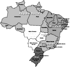
Source: http://www.brasil-turismo.com/geografia.htm.

 

Table 1

Sigh of internal net migration for Brazilian states in the

1995-2000 period

Source: fibge, 2000.

 

Table 2

Proportion of intrastate migrants on the total for Brazilian states in the 1995-2000 period

Source: fibge, 2000.

 

The Center-West Region had the highest values for both types of interstate migration, and the North Region had also a high number for both, indicating that the absorption of population from other Brazilian regions was relatively more effective than the rest of the country, both areas had most of its’ states with positive net migration. Note that the Northeast and Southeast were the ones with the number of migrants between non-neighbors greater than for neighbors. This fact is partially explained by the historically numerous flows between these two macroregions and the strong social nets that were established between them. The South presented the higher values for intrastate migration also due to its’ geographical localization.

Next table discusses the flows of migrants for the four different types –urban-urban, rural-urban, urban-rural and rural-rural– for the period between 1995-2000. Most Brazilian migrants were urban/urban ones, more than 10 millions, or approximately 70% of the total. Following this type of migration, with much smaller numbers, appeared the rural/urban migration, with a little over 2 million migrants, them the urban-rural one and, lastly, the rural-rural migration. These last two with values between 1 and 1.5 million. The urban/urban migration was the most numerous for all the macroregions in Brazil. However, in the North and Northeast regions, the relative values were smaller, because these last two regions had greater proportions of urban/rural and rural/rural migrations than other regions.

 

Table 3

Migrants by distance of migration for macroregions of destiny in the 1995-2000 period

Source: fibge, 2000.

 

Table 4

Migrants by type of migration for macroregions in the 1995-2000 period

Source: fibge, 2000.

 

 

Table 5 presents each type of migration for each kind of distance for Brazil. Note that most migrants for all types of migration were intrastate ones, ranging from 65.6% for urban/urban migration to 80% for rural/rural migration. Notice that the steps of migration were in general shorter for rural/rural migration than the observed for other types. On the other hand, for the urban/urban migration, although most migrants were also intrastate ones, the steps of migration tended to be longer. Notice also that the rural/urban and urban/rural flows were very similar regarding distance, with an intermediate profile. 

This section discussed four types of migration –urban-urban, rural-urban, urban-rural and rural-rural– for three distances –intrastate, interstate between neighbors and interstate between non-neighbors. For more detailed discussions about flows between and within states in Brazil see Golgher (2006a, 2006b). Based on these categories, all the flows in Brazil were analyzed by Cluster Analyses, as presented in the next section.

 

2. Cluster analyses of the flows of migrants

 

This section discusses the regional socioeconomic diversity of 1098 internal flows in Brazil. These flows were obtained by the following methodology. As discussed above, we estimated the origin and destiny matrixes for all states in Brazil, including the intrastate flows, for the four types of flows cited previously. By doing so, we initially obtained a total of 2916 (27 × 27 × 4) flows. Then, for each state as destiny, the interstate between non-neighbors flows were aggregated for each macroregion of origin. Because of its´ population and dimension of the flows, for São Paulo state the flows were all discussed disaggregated by state. The final number of non-zero flows was 1098, which were classified with the use of a multivariate technique of Cluster Analyses.

This technique attempts to identify relatively homogeneous groups of cases based on selected characteristics (Hair et al., 2006). Particularly in this study, we had as objective to classify the flows of migrants in relatively homogeneous groups regarding the following variables: proportion of children (individuals aged 0 to 14 years), proportion of adults (15 to 64 years), proportion of elderly (65 years and above), sex ratio, proportion of married people, proportion of singles, mean schooling level (years of formal education), mean age and mean per capita income. In order to obtain the clusters, we used a decreasing ranking for each one of these variables.

 

Table 5

Migrants by type of migration and distance in Brazil

in the 1995-2000 period

Source: fibge, 2000.

 

There are different techniques to cluster observations (Mingoti 2007) and, among them, the hierarchical and non-hierarchical methods. We chose to use this last method, in particular the K-Means Cluster Analysis Procedure, because it can analyze large data files, and, mostly, due to its ability to save the final cluster centers as an external file, which was a main objective of this paper.

However, this procedure requires the specification of the number of clusters in advance. Due to the amount of information of all the 1098 flows, in order to make the discussion more insightful, the flows were initially divided in five groups, one for each macroregion in Brazil, depending on the destiny. We performed some studies with different numbers of clusters and based on the empirical results, we opted to use the same number for each macroregion, which was six clusters in each analyses.

The results for each cluster final center are shown for each one of the macroregions in tables A1 to A5 in Annex 1, respectively for the North Region, Northeast Region, Southeast Region, South Region and Center-West Region. Notice that the values for each one of the variables are related to its´ ranking among the 1098 flows that we analyzed. Hence, a figure that is close to 1098 indicates that the variable value is amongst the lowest in Brazil. On the other hand, if the cluster center is close to 1, the values are among the highest. The flows of migrants were classified for each one of the macroregions in one of the cluster described in these five tables. The cluster membership for each flow is shown separately for each macroregion of destiny in tables B1 to B5 in Annex 2. Notice that the flows indicated by the Û symbol are between regions, and the flows with Þ symbol are from one origin to a destiny. Note also that the flows are divided among each cluster for the twelve different types of flow, if urban/urban, rural/urban, urban/rural or rural/rural, and if intrastate, interstate between neighbors and interstate between non-neighbors. Given the amount of information, we included one table for each macroregion, tables 6 to 10, with the main results and a summary of the tables in the annexes. Annex 3 gives some explanations in order to facilitate the interpretation of the tables in Annex 2.

 

2.1 North Region

 

All the flows with destiny in the North Region are analyzed in this subsection. Table A1 shows the values for the clusters final centers for each one of the variables. Each cluster is discussed separately in an order that was considered the best one to understanding. 

The cluster number 5 showed higher schooling and income levels than all the other clusters with flows with destiny in the North Region. This can be seen by the lower values for the cluster final centers for these variables, respectively 226 and 248, for this specific cluster. Notice that many clusters in the other tables in Annex 1 had lower values than this one for these variables, indicating that the flows that were categorized in this cluster were among the ones with highest schooling and income levels among the flows with destiny in the North Region, but this is not true if all flows in Brazil are considered. The proportions of adults and married people were also relatively high, as is shown respectively by the values of 110 and 302 for the cluster final centers for these variables. The cluster had also low proportions of children, elderly and singles, as is indicated by the high values of the clusters final centers of these variables, respectively 1,041, 963 and 870. The other variables, sex ratio and median age had values around the national median, as indicated by the values around 550 for final cluster centers. In order to make the discussion more insightful, we included a summary of this information in table 6. The characteristics of this cluster can be summarized as flows: young married adults with high levels of schooling and income.

Table B1 shows which of the flows with destiny in the North Region had these features. The objective of this type of analyses is to present a general profile of the flows and not to discuss a particular one, although this can also be done. Notice that the flows with these characteristics were all interstate between non-neighbors ones, that is, they were long distance steps of migration. Moreover, most flows were urban-urban ones, the majority from the Southeast, South and Center-West regions. The destiny was all over the North Region, with the exception of the states of Pará and of Rondônia. The flows with rural destiny were less numerous. Table 6 also summarizes these main findings from table B1 as follows: long distance flows, mostly with urban destiny, with few flows to Rondônia or to Pará.

The cluster number 3 had schooling and income levels slightly below the cluster above, but still above the others in table A1. The cluster final centers for these two variables were respectively 290 and 269. These two clusters had other similarities, such as: for mean age, that was relatively high; and for the proportion of married people and for the proportion of singles, which were respectively superior and inferior than the other clusters. The most remarkable differences between clusters 3 and 6 is the proportion of children and elderly, much higher in the first one, indicating a greater proportion of nuclear and extended families in cluster 3 when comparing with cluster five, which showed a larger proportion of couples. Table 6 summarizes the features of cluster number 3, as: families with high income and schooling levels.

 

Table 6

Cluster characteristic and main flows – North Region

Source: fibge, 2000.

 

As can be seen in table B1, for cluster 3, similarly to cluster 5, most flows were long distance steps of migration with urban destiny. However, the states of Rondônia and of Pará, contrary to the observed for cluster 5, were the preferential destinies for the flows categorized in cluster 3, and also Tocantins, suggesting that demographic differences did exist for the flows with distinct destinies. Moreover, some flows between neighbors were classified in cluster 3, most also with destiny in Rondônia and Tocantins.

Cluster 1 had schooling and income levels below these first two, but higher than the other remaining three clusters. The characteristics of this cluster were: a low mean age, large proportions of singles and women, and low proportions of married people. Hence, the relatively high levels of education and income were the common features of these three first clusters discussed. However, the first cluster, number 5, characterized young couples, the second, number 3, families, and the third, number 1, young single women.

This last cluster characterized all the intrastate and most urban-urban flows between neighbors. That is, contrary to the long distance flows that showed a larger proportion of families and couples, the short distance urban/urban flows had greater proportions of women and singles. Also note that nearly all urban-urban flows were characterized by one of the three cited clusters, indicating the higher socioeconomic levels of these flows when compared to the other types. 

The other three clusters, numbers 2, 4 and 6, had educational and income levels much inferior than the three above. As can be seen in table B1, these clusters described the main features of most rural/rural flows and the majority among the rural-urban and urban-rural short step flows. That is, there was a clear distinction between these flows and the urban/urban and some of the long distance ones.

Cluster 6 was the one with the lowest levels of education and income among the ones with destiny in the North Region. Besides this, the other main characteristics of the cluster were: the high proportions of children and singles; the very low proportions of adults and married people; and the very low mean age. In other words, as in table 6: families with many children and single adults with low income and formal education. Firstly, no urban/urban flow had these characteristics, namely, all flows had origin and/or destiny in rural areas. Most importantly, this cluster characterized most of the intrastate flows in the North Region that were not urban/urban ones, with the exception of Rondônia state as destiny. Many flows between neighbors, the majority between states in the North Region, were also classified by cluster 6. That is, the flows were intrastate and between neighbors with origin or/and destiny in rural areas, and between non-neighbors with rural destiny.

Cluster 6 is very similar in most aspects to cluster 4. The main difference is that the first had relatively more young singles, while the second had more young married migrants, indicating the dichotomy between single individuals and high fertility families, and family migration. Both clusters categorized many intrastate flows with origin or/and destiny in rural areas, but with one difference: while number 6 classified flows with destiny in the North Region in general, number 4 categorized the flows to Rondônia, indicating a rather different profile for civil status in the flows with destiny in this state.

Cluster 2 showed high proportions of single adults with income and schooling levels slightly above the last two clusters. The proportions of children and of elderly people were very low. Notice that there is a great similarity between this cluster and number 6 in many aspects, such as for: the sex ratio, the proportions of married people and of singles. However, in cluster 2 there was the predominance of single adults, while in cluster 6 there were high fertility families and very young singles. The flows in cluster 2 were all interstate ones with origin and/or destiny in rural areas, mostly long distance flows, showing a rather different profile than cluster 6.

After these explanations about the flows clustering, we include some final commentaries. Firstly, the clusters can be roughly divided in two groups, both characterized many rural/urban and urban/rural interstate migration flows: one with clusters one, three and five, with higher income and schooling levels; and the other with numbers 2, 4 and 6, with lower levels for these variables. The first group also characterized nearly all urban/urban flows, most long distance steps of migration and very few rural/rural flows. The clusters in this group differed among themselves mainly in demographic aspects. Number one was composed especially of singles, but also of families, number 3, of married couples and families, and number 5, consisted mainly of couples. The other group of clusters also differed among themselves mainly due to demographic features: number 2 with single adults; number 4 with families; and number 6 with high fertility families and young flows, with high proportions of singles. These cluster typically characterized short step migration with rural origin or destiny, or rural/rural migration in general.

This same type of discussion will be presented separately for each one of the other four macroregions of Brazil in the same order they appeared in table 1.

 

2.2 Northeast Region

 

The Northeast Region is the one with the lowest socioeconomic levels in Brazil. As is shown in table A2, the values of formal education and income for the flows with destiny in this region were much lower than the national median for five out of six clusters: three of them had rankings for these variables above 900, and the other two over 750.

However, one of them, number 6, had much higher values for both variables, respectively 243 and 244 for the cluster final centers. That is, these flows differed in a great extent in comparison to the others regarding these two variables. All other characteristics of cluster 6 were quite similar to the national median values, that is, they were not decisive while describing this cluster, with slightly low values for the proportions of children, men and singles. Table B2 shows that this profile characterized over 100 flows of migrants, the great majority of the urban/urban type, what clear indicates that the flows between urban centers in the Northeast Region were not preferentially composed of poor people. Besides that, some long distance flows, especially with urban origin or destiny, were classified in this cluster. Table 7 summarizes all the information of tables A2 and B2. 

All the others cluster had very low schooling and income levels and they mainly differed because of demographic features. Cluster 5 characterized very young flows with great proportions of children and singles, and low proportions of adults, elderly and married people, that is to say, high fertility families and singles. The flows were mainly long distance ones, but also between neighbors, mostly with rural origin and/or destiny. This cluster characterized none of the intrastate flows. Moreover, nearly all urban/urban flows that did not follow the features of cluster 6 were classified in this cluster, half with destiny in Maranhão, indicating that the urban/urban profile of this state differed from the rest of the region. 

Cluster 1 had many similarities with cluster 5, such as low levels of income and schooling, high proportions of children and singles, low proportions of adults and married people. One point was the main difference between them: number 1 presents higher proportions of elderly than number 5, what implicates in a higher mean age for this first one. This suggests that the flows in cluster 1 were made of low-income high fertility families and singles, as in cluster 5, and also of elderly people, who might be migrating independently, or perhaps as an extension of the family. This was the profile of most intrastate flows in the Northeast Region, except the urban/urban, which were mostly categorized by cluster 6. Cluster 1 was also the outline of many relatively short distance flows between neighbors in the region, remembering that most states in the region are quite small. These two facts indicate that most or at least a great proportion of flows of migrants with origin and-or destiny in rural areas in the Northeast Region presents the characteristics pointed out by this cluster.

Cluster 4 had as main aspects large proportions of elderly people, especially women, very low schooling and income levels, low proportions of children and high mean age. Notice that the previous cluster also had high proportions of elderly people and low socioeconomic levels. The main difference from number 1 and number 5 is that this last one had much larger proportions of elderly people that tended to be women, possibly widows. Four intrastate urban/rural flows had these characteristics, and also many short distance interstate between neighbors of the urban/rural type, indicating the return of female migrants after retirement or due to life cycle aspects, such as becoming a widow.

Cluster 3 was very similar in many aspects to cluster 5. The socioeconomic levels were similar, namely, very low, as was the proportion of adults. Besides that, the proportions of children were high in both clusters. The main differences between these clusters are that number 3 had higher proportions of elderly people. To be exact, the flows in cluster 3 were represented mostly by low-income high fertility families with elderly people, while in cluster 5, the flows were mostly composed of low-income high fertility families. The flows with the characteristics of cluster 3 were mostly long distance with origin or/and destiny in rural areas. However, notice that the intrastate rural-rural flows in Rio Grande do Norte were categorized in this cluster.

The last cluster to be discussed for flows with destiny in the Northeast Region is number 2, which had socioeconomic levels below the national median, but that showed higher levels of schooling and income than all the other clusters of flows with destiny in this region, but number 6. Cluster 2 had one remarkable feature: great proportions of male adults. Nearly all the flows were long distance ones with rural origin and/or destiny, indicating that a great proportion of these flows was composed of male return migrants after a brief period in the destiny.

Contrary to the observed for the North Region, nearly all urban/urban flows in the Northeast Region were characterized by the cluster with much higher socioeconomic levels than others, indicating that these flows, disregarding the distance, show a much greater similarity among them than the other flows with destiny in the Northeast Region.

Moreover, notice that in all tables in Annex 1 only three clusters had values above 900 for cluster final centers for income and schooling among the 30 clusters discussed for all macroregions in Brazil. All of them had as destiny the Northeast Region. Other two clusters, one with destiny in the Northeast Region and another with destiny in the North Region had values above 840 for these same variables. Explicitly, these were the flows of migrants with the larger proportions of poor people in Brazil. Besides this similarity in socioeconomic levels, among the four clusters with destiny in the Northeast Region with very low socioeconomic level, the demographic distinctions were remarkable: one had large proportions of elderly women, number four; another had extremely low mean age, cluster five, including high fertility families; other, cluster 3, was composed mainly of families; and lastly, cluster 1, with flows with large proportions of children and elderly people, indicated extended families and complex flows. 

      

2.3 Southeast Region

 

This subsection discusses the results for flows with destiny in the Southeast Region. Two clusters, numbers 5 and 6, as shown in table A3, presented much higher socioeconomic levels than most of the ones discussed above. The presentation will begin with this last cluster, the one with the highest levels of schooling and income for flows with destiny in this region, respectively with ranking values of 192 and 208 for the cluster final center. Notice also that this cluster had the second highest value among the 30 cluster discussed for all the five macroregions in Brazil, losing only to number 4 in the South Region, indicating that the flows characterized by it were among the most prosperous in Brazil. The other main characteristics of cluster 6 were the low proportions of children, of singles and men, and high proportions of adults. In other words: low fertility high-income families and women with high income and schooling levels. These were the characteristics of most urban/urban flows with destiny in the Southeast Region, including all the intrastate ones. Cluster 6 also categorized very few other flows of the rural/urban or urban/rural types.

Cluster 5 had socioeconomic levels slightly lower than the cluster above and had also low proportions of children. The main difference between these two clusters was the much higher proportions of men and adults in cluster 5. Rather differently than the cluster above, all the flows had rural origin and/or destiny, mostly long distance flows, indicating the relative higher attraction of rural areas for men, especially in the states of Rio de Janeiro and São Paulo, including individuals with high income.

These two clusters had much higher socioeconomic levels than the others, well above the national median. All the other clusters had values around the Brazilian median. Cluster 1 presented low proportions of children, of elderly, of men and of married people, and high proportion of adults and singles. The flows were also very young. That is, mainly young female adults with medium levels of income and schooling. All the urban-urban flows that were not classified in cluster 6 were categorized by cluster 1. Notice that most of then had as origin the North or Northeast regions, the two poorest in Brazil. Moreover, flows from these two regions, but with rural origin and/or destiny also were categorized by this cluster, mostly long distance flows. Rio de Janeiro and São Paulo were the main destinies, indicating the power of population attraction of these areas over the young females of the North or the Northeast of Brazil.

 

Table 7

Cluster characteristic and main flows – Northeast Region

Source: fibge, 2000.

 

Cluster 2 had as its´ main characteristics the high proportions of elderly people, which was the highest one among all the 30 clusters in Brazil, high proportions of females and low proportions of adults and singles. Cluster 4 had the same socioeconomic levels as cluster 2, but with higher proportions of men, adults and married people. Namely, in the first cluster old women predominated and in the last one, the same occurred for low fertility families. These are the features of many flows with rural origin or/and destiny, including nearly all intrastate flows in the Southeast Region. However, which one is the main difference regarding the composition of the flows between these clusters? They show many similarities, but some differences can also be noted. Cluster 2 shows a greater proportion of urban/rural flows, probably many return migrants, including the two most rural states of the region Minas Gerais and Espírito Santo. Cluster 4, although also with many urban/rural flows, showed a greater number of rural/urban and rural/rural flows, especially intrastate and short distance ones.

Cluster 3 had the lowest socioeconomic levels in the Southeast Region, but still the values were just slightly below the national median. The flows presented as main features a very low mean age, with great proportions of children and low proportions of adults and elderly people. These main features can be summarized as: medium income high fertility families. The flows were mainly long distance ones with rural origin and-or destiny. This fact was also observed for cluster 5. However, these clusters had some remarkable differences in socioeconomic and demographic features, and also in the origin of the flows. In cluster 3, the origin was mainly the Northeast, North and Center-West regions, with relative higher proportions of high fertility low/medium income families, while for cluster 5, the origin was mostly the South Region, with high-income people with lower levels of fertility.

 

2.4 South Region

 

Table A4 shows the characteristics of the clusters regarding the flows with destiny in the South Region. These flows, as was also observed for the Southeast Region, had schooling and income levels above the national median, especially two of the clusters, numbers 2 and 4. As mentioned, this last cluster had the highest levels of schooling and income in Brazil. Besides that, the proportions of singles were smaller, with one exception, that is cluster 6, and the proportions of married people were higher, with two exceptions, clusters numbers 2 and 6, than the Brazilian values. These aspects indicated overall differences in socioeconomic, age and civil status between the flows with destiny in the South Region and the others in Brazil.

The two clusters with higher socioeconomic levels, numbers 2 and 4, mostly this last one, characterized all the urban/urban flows. Moreover, this last cluster had as its´ main characteristics the low proportions of children and of singles, and the high mean age. That is, they were mainly high-income low fertility families. Although the flows were mostly urban/urban ones, some long distance rural/urban and a few urban/rural flows were also observed with these features.

Cluster 2 had socioeconomic levels that were slightly lower than cluster 4, but still remarkably elevated. These two clusters differed mainly in demographic aspects, such as: greater proportions of children, of women and of singles in cluster 2, which also had a lower mean age. That is to say, the families had higher levels of fertility and single young females were more present in the flows categorized by this cluster. The flows that had these characteristics were mostly urban/urban with Paraná as the destiny, and rural/urban and urban/rural, with Rio Grande do Sul as destiny. 

Two clusters characterized nearly all the intrastate flows with rural origin and/or destiny: numbers 5 and 3. Both had schooling and income levels around the national median, much lower levels than the two clusters above. Both had also very low proportions of singles and very high proportions of married people. Cluster 5 had relatively low proportions of children and high ones of elderly, while the contrary occurred with number 3. In other words: cluster 5 was composed mostly of couples with high mean age, with few siblings, while cluster 3 characterized mostly families with children. All the flows in both cluster had rural origin and/or destiny. The main difference was the origin of the flows: for cluster 5, they were the North and Northeast regions; and for cluster 3, were from the other regions in Brazil.

The two last clusters for flows with destiny in the South Region, numbers 1 and 6, had mean values for schooling and income, low mean age and low proportions of elderly people. The main differences between them were that cluster 1 had a predominance of women and greater proportions of married adults, while cluster 6 showed a predominance of men and greater proportions of singles and children. Namely, the first one was composed preferentially of young medium-income low fertility families with female predominance, while the second characterized mostly flows with young adults with male prevalence. Both characterized mainly long distance flows with origin and/or destiny in rural areas with similar origins and destinies.

 

2.5 Center-West Region

 

Tables A5, B5 and 10 show the results for the flows with destiny in the Center-West Region. As can be seen in the first one of these tables, three clusters had schooling and income levels above the national median, numbers 1, 2 and 5, two had values around the Brazilian median, numbers 3 and 6, and just one had values below this, that was cluster 4. Table B5 presents a general picture that is less clear than the observed for other regions, although a regularity for intrastate flows are noticeable. Observe that the intrastate flows for the Federal District do not exist.

 

Table 8

Cluster characteristic and main flows – Southeast Region

Source: fibge, 2000.

 

Beginning the discussion with the clusters with higher socioeconomic levels, what are the main differences between clusters 1, 2 and 5? Cluster 1 had as its main features the very high proportions of children, very low proportions of adults and elderly people and very low mean age. Cluster 2 had low proportions of children and singles and high proportions of married people. Cluster 5 presented all demographic variables around the mean. Concluding, the relative high-income flows with destiny in the Center-West Region were divided in three groups: high fertility families; couples; and families. All these clusters categorized very few rural/rural flows, that is, most had urban origin and/or destiny. The flows of cluster 1 had as destiny Mato Grosso and Mato Grosso do Sul, areas, especially the first of these states, of recent significant absorption of immigrants due to its´ location in the south fringe of the Amazon forest. On the other hand, many flows with cluster 2 characteristics had Goiás as destiny, including the rural/urban and urban/rural intrastate flows. The cluster number 5 characterized most short distance urban/urban flows, including the three intrastate ones, and most interstate between neighbors.

Two clusters, 3 and 6, had medium levels for schooling and income. They also showed small proportions of children and of elderly and high proportions of adults. Cluster 6 was the “oldest” in Brazil, although the proportion of elderly was not so high. This indicates that the adults were not young, even though they were not yet considered aged. The cluster had large proportions of married people, with predominance of men. Cluster 3 differed from the previous in four main aspects: the mean age was much lower, the proportions of singles were much smaller; the contrary was observed for married people; and the predominance of women was much greater. In a few words: married couples relatively aged with slight prevalence of males for cluster 6; and young single adults with predominance of females for cluster 3; all with medium income and schooling levels. Both clusters characterized only interstate flows. Moreover, very few flows were characterized by cluster 6, mostly rural/rural long distance from the South or Southeast regions, signaling the return of migrants. Cluster 3 categorized also mostly long distance flows, but especially with urban origin and/or destiny with origin in the North or Northeast regions, indicating a rather different profile. 

 

Table 9

Cluster characteristic and main flows – South Region

Source: fibge, 2000.

 

The last cluster to be analyzed is number 4, with much lower levels of income and education than the others with destiny in the Center-West Region. The other main feature of the cluster was male predominance. The flows with these characteristics were short distance with rural origin or/and destiny, including most intrastate flows. Some long distance rural/rural type were also observed, especially with origin in the Northeast and North regions, indicating the lower socioeconomic status of these flows, when compared to others with destiny in the region.

 

3. Final discussion and conclusions

 

We have presented some of the characteristics of all intrastate and interstate flows of migrants in Brazil. In order to analyze the main similarities and differences between them, we have used the multivariate technique of Cluster Analyses. We have clearly observed some general trends, such as: the higher socioeconomic levels of the urban/urban flows; the lower income and schooling levels of the rural/rural ones; long distance flows tended to present higher values for these variables than short ones; females tended to predominate in flows with urban origin and/or destiny and males were the majority in many rural/rural flows; married people predominated in many long distance flows, while singles dominated short step migrations.  

Although some general trends could be noticed, we have observed that the flows main features were highly context dependent, and the heterogeneity was quite large. However, it was noticed that the poor migrants concentrated in rural/rural, rural/urban and urban/rural flows with destiny in the North or Northeast regions, especially this last one, including long distance flows.

Despite the many aspects that link migration, income and poverty, migration appears to be mainly an ex-ante strategy (Ghobadi et al., 2005). De Haan (1999) observed that most studies that analyzed regional development did not give the appropriate importance to migration. Human mobility is much more common than normally assumed by the notion that population is essentially sedentary. Therefore, given the importance of migration, policies that promote mobility or that increase the positive effects of migration should be encouraged, including policies that diminish the costs of migration, which would have a positive impact on the range of possibilities for the low-income population strata. For instance, policies that: improve channels for information exchange; facilitate the absorption of the migrant in the destiny; minimize environmental damages; increase the effectiveness of the use of remittances for local development, are some examples.

It must be emphasized that these policies tend to present a multiplicative effect due to positive externalities and herd effects (Bauer et al., 2002). Previous migrations tend to further diminish the costs of currently migration, as, normally, individuals migrate to places where they receive general assistance from others migrants via social nets, and/or where other migrants already live. Besides that, this preceding migration stands as a quality of life signal of the potential destiny, lowering the costs of information transaction.  

 

Table 10

Cluster characteristic and main flows-Center-West Region

Source: fibge, 2000.

 

Annex 1

 

Table A1

Clusters final centers for flows with destiny in the

North Region

 

Table A2

Clusters final centers for flows with destiny in the

Northeast Region

 

Table A3

Clusters final centers for flows with destiny in the

Southeast Region

 

Table A4

Clusters final centers for flows with destiny in the South Region

 

Table A5

Clusters final centers for flows with destiny in the Center-West Region

 

Annex 2

 

B1- Flows categorization in clusters – North Region

 

B2 - Flows categorization in clusters – Northeast Region

 

B3 - Flows categorization in clusters – Southeast Region

 

B4 - Flows categorization in clusters – South Region

 

B5 - Flows categorization in clusters – Center-West Region

 

Annex 3

 

 

References

 

Barros, Ricardo, Ricardo Henriques and Rosane Mendonça (2000), “A estabilidade inaceitável: desigualdade e pobreza no Brasil”, in: Ricardo Henriques, Desigualdade e pobreza no Brasil, ipea, Rio de Janeiro, pp. 21-47.

 

Bauer, Tomas, Gil Epstein and Ira Gang (2002), “Herd effects or migration networks? The location choice of Mexican immigrants in the U.S.”, Discussion Paper 551, Institute for the Study of Labor, Bonn.

 

Bell, Paul, Jeffery Fisher, Andrew Baum and Thomas Greene (1990), Environmental psychology, Harcourt Brace Jovanovich College Publisher, Forthworth.

 

Borjas, George (1987), “Self-selection and the earnings of immigrants”, America Economic Review, 77 (4), American Economic Association, Nashville, pp. 531-553.

 

Borjas, George (1998), “The economic progress of immigrants”, nber Working Paper Series, n. 6506, Cambridge, http://www.nber.org/papers/w6506. 

 

Cadwaller, Martin (1992), Migration and residential mobility: macro and micro approaches, The University of Wisconsin Press, Madison.

 

Carvalho, Jose and Claudio Machado (1992), “Quesitos sobre migrações no Censo Demográfico de 1991”, Revista Brasileira de Estudos Populacionais, 9 (1), Associação Brasileira de Estudos Populacionais, Rio de Janeiro, pp. 22-34.

 

Castiglioni, Aurélia (1989), Migration, urbanisation et développement: le cas de l’Espírito Santo-Brésil, Ciaco Editeur, Pouvan.

 

Ferreira, Francisco, Peter Lanjouw and Marcelo Neri (2000), A new poverty profile for Brazil using ppv, pnad and census data, puc, Rio de Janeiro.

 

fibge (2000), Censo Demográfico do Brasil, ibge, Rio de Janeiro.

 

Ghobadi, Negar, Johannes Koettl and Renos Vakis (2005), “Moving out of poverty: migration insights from rural Afghanistan”, www.mrrd.gov.af/vau/.

 

Golgher, André (2006a), Diagnóstico do processo migratório no Brasil 2: migração entre estados, Cedeplar-ufmg, Belo Horizonte.

 

Golgher, André (2006b), Diagnóstico do processo migratório no Brasil 3: tipos de migração, Cedeplar-ufmg, Belo Horizonte.

 

Haan, Arjan de (1999), “Livelihoods and poverty: the role of migration – a critical review of the migration literature”, The Journal of Development Studies, 36 (2), abi-inform Global, Routledge, Florence, Kentucky, pp. 1-47.

 

Hagen-Zanker, Jessica and Mirtha Castillo (2005) “Remittances and human development: the case of El Salvador”, Working Paper, Maastricht Graduate School of Governance.

 

Hair, Joseph, Rolph Anderson, Ronald Tathan and Willian Black (2006), Analise Multivariada de Dados, Bookman, Porto Alegre.

 

Hoffmann, Rodolfo (2000), “Mensuração da desigualdade e da pobreza no Brasil”, in Ricardo Henriques, Desigualdade e pobreza no Brasil, ipea, Rio de Janeiro, pp. 81-107.

 

ibre-fgv (2005), Miséria em queda: mensuração, monitoramento e metas, Centro de Políticas Públicas do ibre-fgv, Rio de Janeiro.

 

Kothari, Uma (2002), Migration and chronic poverty, idpm-Chronic Poverty Research Centre, Manchester.

 

Massey, Douglas, Joaquim Arango, Graeme Hugo, Ali Kouaouci, Adela Pellegrino and John Taylor (1998), Worlds in motion: understanding international migration at the end of the millennium, Clarendon Press, Oxford.

 

Rigotti, Irineu and José Carvalho (1998), “As migrações na grande região centro-leste”, Encontro Nacional sobre migração, 1, ipards-fnuap, Anais, Curitiba, pp. 67-90.

 

Rigotti, Irineu (1999), “Técnicas de mensuração das migrações a partir dos dados censitários: aplicação dos casos de Minas Gerais e São Paulo”, Tese (Doutorado em Demografia), cedeplar, Belo Horizonte.

 

Sandefur, Gary, Nancy Tuma and George Kephart (1991), “Race, local labor markets, and migration, 1975-1983”, in John Stillwell and Peter Congdon (eds.), Migration models: macro and micro approaches, Belhaven, London-New York, pp. 187-206.

 

Stark, Oded (1991), The migration of labor, Blackwell Publisher, Chichester, West Sussex.

 

Stillwell, John and Peter Congdon (1991), “Migration modeling: concepts and contents”, in John Stillwell and Peter Congdon (eds.), Migration models: macro and micro approaches, Belhaven, London-New York, pp. 1-16.

 

Todaro, Michael (1980), “Internal migration in developing countries: a survey”, in Richard Easterlin (ed.), Population and economic change in developing countries, University of Chicago Press for the National Bureau of Economic Research, Chicago, pp. 361-390.

 

Vasconcelos, Pedro (2005), Improving the development impact of remittances, United Nations Expert Group Meeting on International Migration and Development, New York.

 

Waddington, Hugo and Rachel Sabates-Wheeler (2003), How does poverty affect migration choice? a review of literature, Development Research Centre on Migration, Globalization and Poverty-University of Sussex, Brighton.

 

 

Recibido: 3 de abril de 2007.

Reenviado: 20 de abril de 2009.

Aceptado: 19 de mayo de 2009.

 

André Braz Golgher. Es doctor por el Centro de Planeamiento y Desarrollo Regional de la Universidad Federal de Minas Gerais (ufmg), Brasil. Realizó sus estudios de licenciatura en física y la maestría en química en la misma universidad. Actualmente es profesor del Centro de Planeamiento y Desarrollo Regional en el Departamento de Economía. Sus líneas de investigación actuales son: migración, pobreza y educación. Entre sus publicaciones destacan: em coautoría, Matemática: questões da anpec resolvidas 1993-2007, ufmg, Belo Horizonte (2008); en coautoría, “The determinants of migration in Brazil: regional polarization and poverty traps”, Papeles de Población, 56, México, pp. 135-171 (2008); en coautoría, “Human capital differentials across municipalities and states in Brazil”, Population Review, 47, Project muse®, Baltimore, p. 2, (2008).

 

Denise Helena França Marques. Realizó sus estudios de licenciatura en economía en la Universidad Federal de Minas Gerais (ufmg) y actualmente es estudiante de doctorado en el Programa de Posgrado en Demografía del Centro de Planeamiento y Desarrollo Regional (Cedeplar-ufmg). Fue investigadora en el Proyecto Nacional sobre Diversidad en la Escuela, así como consultora para el Fondo de Población de las Naciones Unidas (unfpa), Brasil. Sus áreas de interés son: migraciones internacionales, movimientos circulares en fronteras nacionales, comunidades transnacionales y brasiguaios. Entre sus publicaciones destacan: “Sustentabilidade e condições de vida em áreas urbanas: medidas e determinantes em duas regiões metropolitanas brasileiras”, eure, xxxii, Santiago, pp. 47-71 (2006); “Wage differences between the so called “brasiguaios” and the Brazilian emigrants coming back from United States; an application of counter-factual migro-simulation”, in International Conference Moscou, Migration and Development, v. ii pp. 233-253, (2007); “As grandes metrópoles e as migrações internas: um ensaio sobre o seu significado recente”, in Anais do IV Encontro Nacional sobre Migrações, iv Encontro Nacional sobre Migrações, Rio de Janeiro (2005).